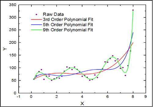
Polynomial regression is ordinary least squares regression with polynomial feature expansion to introduce nonlinearity. For univariate data, the columns of the design matrix become:

\bf{X} = \left[\begin{matrix} \bf{1} & \bf{x} & \bf{x}^2 & … & \bf{x}^p \end{matrix}\right]

We’re working with the univariate smooth synthetic data in this experiment, so there is no possibility for interaction terms in our polynomial expansion.

Elastic Net Regularization

Elastic net regularization reduces overfitting by penalizing large coefficients, which makes the curve smoother. The penalty is the sum of two traditional regularization penalties taken from LASSO and ridge regression.

L₂-norm

Also known as ridge regression or Tikhonov regularization, using this quadratic penalty term especially helps avoid overfitting when features are correlated. It penalizes the sum of the squared coefficients:

\left\lVert \bm{\beta} \right\rVert_2^2 = \sum_j \beta_j^2

This is the same as imposing a Gaussian prior \mathcal{N}(\beta | 0, \lambda^{-1}) where \lambda is a positive number indicating the strength of our belief that \beta should be close to 0. L₂-norm regularization is convenient because it retains a closed-form solution to the minimization problem.

L₁-norm

Also known as LASSO (least absolute shrinkage and selection operator), this method of regularization forces some coefficients to zero. This leads to a sparse model, making it a form of feature selection. It penalizes the sum of the absolute value of the coefficients:

\left\lVert \bm{\beta} \right\rVert_1 = \sum_j | \beta_j |

The L₁-norm is not differentiable, so there is not a closed form solution. However, the cost function is still convex and can be solved through iterative methods.

LASSO can be interpreted as linear regression for which the coefficients have Laplace prior distributions, sharply peaked at zero.

Putting it Together

The complete polynomial regression with elastic net regularization formula with weights is:

\min_{\bm{\beta}} \sum_i w_i (\bf{X}_i \bm{\beta} - y_i)^2 + \lambda_2 \left\lVert \bm{\beta} \right\rVert_2^2 + \lambda_1 \left\lVert \bm{\beta} \right\rVert_1

Experiment Design

For our tests on univariate smooth, we use:

• sklearn.preprocessing.PolynomialFeatures to generate the design matrix
• sklearn.linear_model.ElasticNet for the modeling
• skopt.forest_minimize to optimize the hyperparameters

We have three hyperparameters to optimize:

• degree: max polynomial degree during feature expansion
• alpha: equivalent to \lambda_1 + 2 \lambda_2
• l1_ratio: equivalent to \lambda_1 / (\lambda_1 + 2 \lambda_2)

The hyperparameter search space is:

• degree: integer drawn uniformly from [1, 10]
• alpha: real value drawn from log-uniform distribution with base 10 from [1e-6, 1e-1]
• l1_ratio: real value drawn uniformly from [0, 1]

We run the hyperparameter optimization routine with 50 calls to an objective function, which itself uses 3-fold cross-validation. We run the hyperparameter optimization routine 25 times on new synthetic datasets, for each of the following dataset sizes growing by powers of 2:

2**13       8,192
2**14      16,384
2**15      32,768
2**16      65,536
2**17     131,072
2**18     262,144
2**19     524,288
2**20   1,048,576
2**21   2,097,152
2**22   4,194,304
2**23   8,388,608

So, we run a lot of regressions to evaluate this machine learning method: 3 \times 50 \times (25 + 1) \times 11 = 42900.

Results

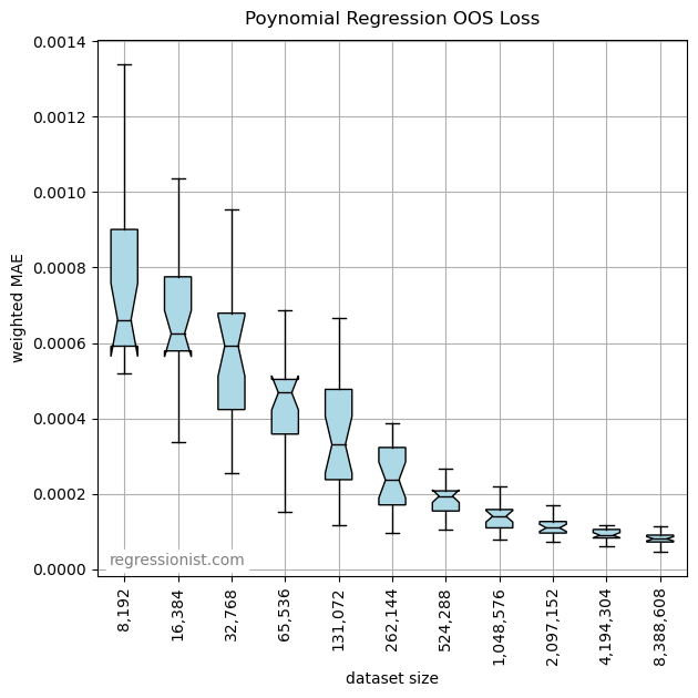
So, it looks like you really need several million samples in the training data to get a good fit. Here is an example fit from the largest dataset size:

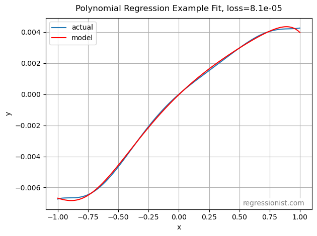
To get this plot, the parameters and values are:

samples = 8388608
degree = 10
alpha = 1.05e-06
l1_ratio = 0.191
loss = 8.13e-05
coeff for power 0 = -2.31e-05
coeff for power 1 = 0.00748
coeff for power 2 = -0.00373
coeff for power 3 = 0.00108
coeff for power 4 = 0.00228
coeff for power 5 = -0.00334
coeff for power 6 = 0.00144
coeff for power 7 = -0
coeff for power 8 = 0
coeff for power 9 = 0.00011
coeff for power 10 = -0.00132

Concerns

Those fit coefficients are similar in magnitude. That is probably due to the use of L₂-norm regularization which really penalizes large coefficients.

The analytical solution for ridge regression is:

\bm{\beta} = (\bf{X}^T \bf{X} + \lambda \bf{I})^{-1} \bf{X}^T \bf{y}

where \bf{I} is the identity matrix. It is called “ridge” regression because of the shape along the diagonal of \bf{I}. We are adding positive elements to the diagonal of the Gram matrix, decreasing its condition number. Our concern is that we’re adding a constant value to the diagonal. It might make more sense to proportionally scale the elements of the diagonal. Our design matrix \bf{X} has extremely small values in the high-degree columns. If the high-degree columns were as important as the low-degree columns, then they would need large coefficients to compensate. And those aren’t easy to get with ridge regression.

Standardization

The easiest way to solve our problem is to standardize the design matrix after expanding the features. For that we use sklearn.preprocessing.StandardScaler. to subtract the mean and divide by the standard deviation of each column (except the first column of ones). Now the Gram matrix should have the same value along the diagonal, and the L₂-norm penalty will be applied equally to each polynomial feature.

Results with Standardized Features

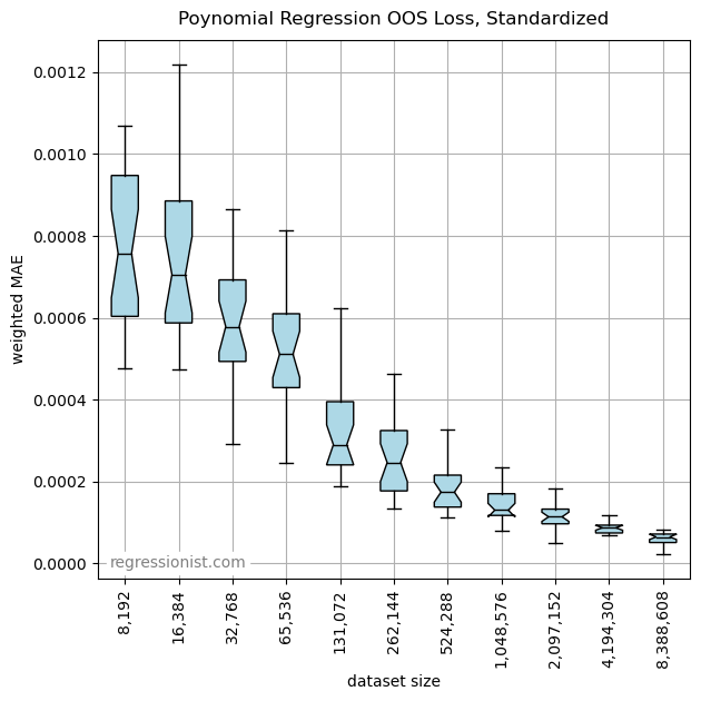
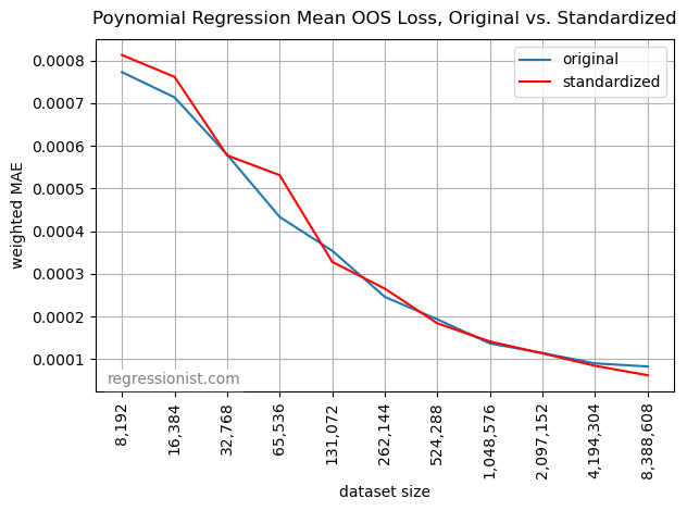
It isn’t clear that standardization made it any better. It penalizes high-degree features less, which hurts for small datasets and helps a little for the largest datasets. Here is a plot of the mean losses from both boxplots:

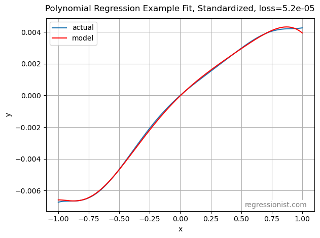
Here is an example standardized fit from the largest dataset size, showing a little tighter fit at the extremities:

Conclusion

It wouldn’t normally seem like a good idea to use a 10-degree polynomial to fit noisy data. But with enough data and regularization it actually turned out quite well. There are more directions we would like to take with this model, but that will have to wait. We are more anxious to explore other regression methods.