XGBoost–short for eXtreme Gradient Boosting–is a powerful boosted decision tree algorithm that has become quite popular due to its winning performance in many Kaggle competitions.

XGBoost is an example of ensemble modeling and creates predictions from a combination of many smaller decision trees. XGBoost also (as implied by the name) implements boosting, where each new tree made reduces the errors of previous trees.

At iteration t and for an observed value y_i with predicted value \hat{y}_i , the algorithm minimizes the following function by adding the new tree f_t that best improves the model:

\text{Objective} = \sum_{i=1}^n l(y_i, \hat{y}_i^{(t-1)} + f_t(x_i)) + \Omega(f_t)

where l measures model accuracy on training data and \Omega is the regulating term that penalizes model complexity.

XGBoost has a long list of hyperparameters. We focus on a few common ones in our model tuning:

• max_depth: maximum depth of a tree with a default value of 6. We search uniformly on the interval [3,10] .
• eta (learning rate): scales the weights of new features. We search [0,1] .
• lambda: L2 regularization term on weights. Our search space is [0,2] .
• alpha: L1 regularization term on weights with a default of 0. We consider [0,2] .
• subsample: the fraction of data samples used in each tree. We search on [0.0001,1] .
• colsample_bytree: the fraction of columns or features sampled for each tree. We search the interval [0,1] .

We also pay some special attention to this parameter:

• objective: the loss function used by the XGBoost algorithm. Options include reg:squarederror and reg:pseudohubererror.

Experiment Design

Here we test XGBoost on the multivariate interaction dataset which has nonlinear data composed of many features.

In order to optimize our hyperparameters, we use skopt.forest_minimize. We do this by performing 50 calls to an objective function that uses 3-fold cross-validation. We run the optimization routine on 25 new synthetic datasets of each dataset size from 2^{13} growing by powers of two to 2^{24} in order to compare prediction errors between dataset sizes.

XGBoost allows the use of different loss functions. We run a second test by creating 25 models on datasets of size 2^{19} using both the ‘reg:squarederror’ and the ‘reg:pseudohubererror’ options and compare the results.

Results

Here we see a boxplot of performance of the algorithm as dataset size increases:

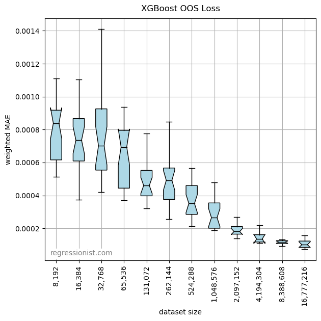
This is a reasonable model, but we do see that in order to produce a high level of accuracy, we need a lot of data.

XGBoost also allows generation of a plot of feature importance. Here are the results from a model created on our largest dataset size:

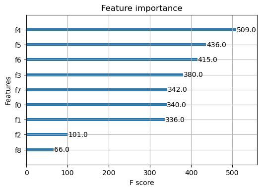
Remembering that f6 , f7 , and f8 are superfluous features, we see that XGBoost correctly dismisses f8 as the least important feature but does give significant weight to f6 and f7 .

We also see the comparative results of using squared error in our model creation compared to using a Huber loss function:

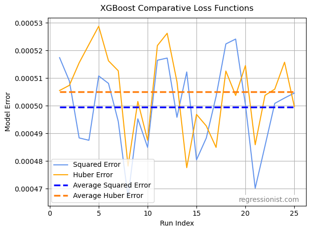
For this dataset, it is in our favor to use XGBoost’s ‘reg:squarederror’ as our option for the objective parameter. These model errors also highlight the importance of parameter tuning. By examining our previous boxplot, we see that each of these non-optimized models appears to have an error score somewhere in the worst 25% of error scores for models previously constructed on the same dataset size with optimized parameters.

Conclusion

XGBoost is certainly a competent algorithm and provides some handy tools, such as the ability to plot feature importance. That being said, its ability to handle superfluous features was mediocre, as it failed to recognize two of our three meaningless features.

Our experimentation on loss functions shows that a squared loss function is better than Huber loss on this particular dataset–an observation that will benefit us as we continue exploring machine learning algorithms for complicated data with many features.