Gaussian process regression (also called kriging) is a form of Bayesian machine learning that forms a model based on a prior distribution and observed data. It is so named because of the Gaussian distribution from which functions are sampled in model creation.

With training data as input, all functions that model the data (with some noise tolerance) are considered and given a probability score based on how likely that function is to be the true model. The functions to be sampled from the prior distribution are chosen by a kernel function (similar to the kernel used in support vector machines). Different kernels have different attributes or strengths, and kernels can be combined by the use of addition, multiplication, or other operations for use in different circumstances. Some examples are the following:

• Radial-basis function (RBF) kernel: a frequently used kernel good for generating smooth functions. Here the function d represents Euclidean distance and l is the length-scale hyperparameter.
  k(x_i, x_j) = \exp\left( -\frac{d(x_i, x_j)^2}{2l^2} \right)
  
• Rational quadratic kernel: essentially a summation of many RBF kernels with different length scales. The parameter l once again is the length scale and \alpha is the scale mixture parameter.
  k(x_i, x_j) = \left( 1 + \frac{d(x_i, x_j)^2}{2\alpha l^2} \right)^{-\alpha}
  
• Periodic kernel: used for functions that include repeating patterns (e.g. weather data). The variable p is the periodicity parameter and determines the distance between repetitions in the function.
  k(x_i, x_j) = \exp\left( -\frac{2\sin^2(\pi d(x_i, x_j)/p)}{l^2} \right)
  
• Dot-product kernel: can be used in combinations for Bayesian polynomial regression. The hyperparameter \sigma_0^2 puts a prior on the y-intercept of the function. This is a linear kernel when \sigma_0^2 = 0.
  k(x_i, x_j) = \sigma_0^2 + x_i \cdot x_j
  

Other kernels options include constant kernels for scaling and white kernels for noise handling.

When test data is added, the distribution of functions is refined to become more precise and have a smaller confidence interval:

p(f|y_i) = \frac{p(f,y_i)}{p(y_i)}

In other words, the probability of a function f given a new observation y_i is equal to the probability of the function and the point divided by the probability of observing that point at the input. This is known as “conditioning” because test points are conditioned on training data. In this way a Gaussian distribution is predicted at each test point.

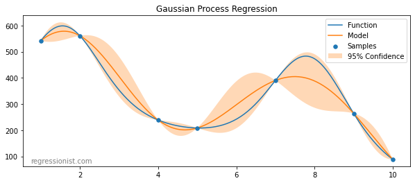
The final function chosen as the model is the mean of functions from the posterior distribution. One useful and cool feature of the Gaussian process is that because functions are taken from a distribution with mean and standard deviation, we also obtain a confidence interval around the model function.

In this experiment we use the scikit-learn implementation of Gaussian process regression.

Experiment Design

We test the effectiveness of Gaussian process regression on the univariate smooth dataset. One handy feature of the scikit Gaussian process algorithm is that it automatically tunes hyperparameters of the kernel used. We create 25 tuned models on synthetic datasets of size 2^{13}. We then increase the dataset size by a power of two and create 25 additional models on new datasets of that size and continue the pattern for a day on a server with 256 GB RAM. We allow the code to complete as many rounds as possible throughout the day.

We use a standard radial-basis function (RBF) kernel (to aid in creating a smooth function) combined with a white kernel by summation (for handling of noise).

Results

After running for a day, the code finished three rounds of modeling. Here we observe the error for models of size 2^{13}\rightarrow 2^{15}:

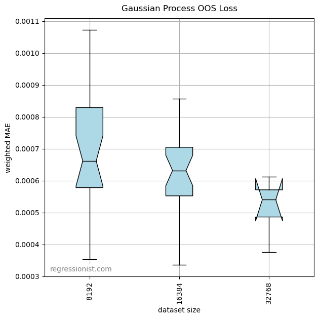
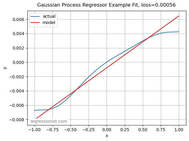
Below is an example fit from our largest dataset size. It provides a reasonable fit, although it has not found a better model than a linear one:

Conclusion

Gaussian process regression has reasonable but not exceptional results on this data. The algorithm runs slowly and uses a lot of memory. Similar experiments on the same dataset were able to complete testing through datasets over twice as large (and sometimes even 8 or 16 times as large) in a roughly equivalent amount of time.

The built-in parameter optimizing makes it handy for creating a model without writing code for tuning but designing an appropriate kernel can be time consuming. The results of the model (though not better than linear) are similar to other algorithms for regression on this amount of data. Perhaps the biggest and most interesting benefit of Gaussian process regression is that it provides the standard deviation and allows the formation of confidence intervals.