Support vector machines (SVMs) are well-known for classification problems. Here we apply the regression method — Support Vector Regression (SVR). The SVM software we use here comes from scikit-learn.
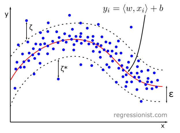
In SVR algorithms, a kernel function maps datapoints to a higher dimension, which helps lower computational cost. We provide a value \epsilon, and the algorithm performs regression in the higher dimension to obtain a hyperplane of least error with a margin of width \epsilon. Values within the \epsilon-tube of the hyperplane are not penalized, and those outside are penalized.
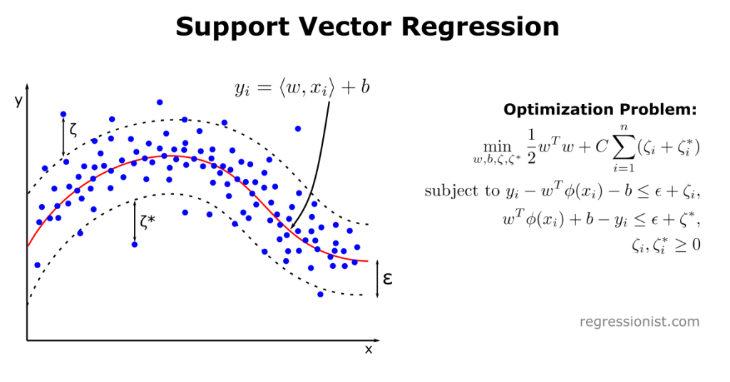
In this illustration, C is the regularization parameter and \phi is the kernel function. The variable \zeta is known as the slack variable, which is the distance a datapoint is from the \epsilon-tube. Note that \zeta_i = 0 if x_i is below the upper bound of the \epsilon-tube and \zeta_i^* = 0 if x_i is above the lower bound of the \epsilon-tube.
One useful and interesting feature of SVMs is the ability to use different kernels for the decision function. Here we test the SVR implementation with the Radial Basis Function (RBF) kernel, which is defined as follows:
RBF: \exp(-\gamma||\bm{x}-\bm{x}'||^2)
Here \gamma is the hyperparameter ‘gamma’ that is discussed below.
Experiment Design
We want to see how SVR handles noisy data from the univariate smooth dataset. In our test, we optimize our hyperparameters using sci-kit’s skopt.foest.minimize, but as an alternative, one may use the built in GridSearchCV and RandomizedSearchCV in tuning.
We optimize the following hyperparameters for SVR with the RBF kernel by drawing from a log-uniform distribution with base 10:
- C: the regularization parameter. C is 1 by default, with lower values making a simpler decision function at the cost of accuracy and higher values making a more exact fit at the risk of overfitting. We search the interval [0.1, 100].
- gamma: used in the RBF kernel decision formula. This parameter defines the influence of a single training example. The larger gamma is, the smaller the radius of influence of a training example. We draw from the interval [1e-4, 10].
- epsilon: defines the size of the epsilon-tube where predicted values within epsilon of the actual values are not penalized during training. We search within [1e-5, 0.1].
We perform the hyperparameter optimization process with 50 calls to an objective function that uses 3-fold cross-validation. We run the optimization routine 25 times on new synthetic datasets growing in size by powers of two from 2^{13}\rightarrow2^{16}.
Ideally, we would continue to test datasets of larger sizes, but we are unable to scale the SVR algorithm on our cluster because of its high computational complexity.
Results
We first look at the error for models of increasing dataset sizes:
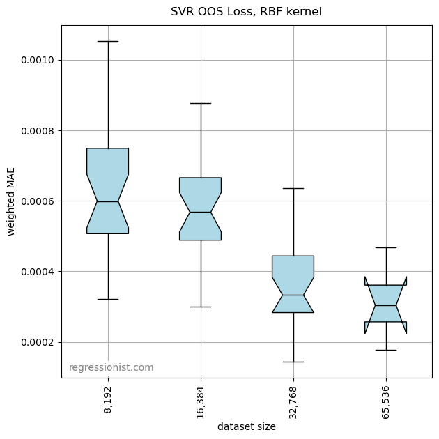
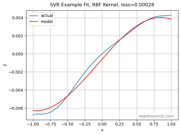
This algorithm outperforms both gradient boosting and polynomial regression for these dataset sizes on the univariate smooth dataset. Here we see an example fit for our largest dataset size:
Conclusion
While its counterpart SVC algorithm is already well-known, SVR performs very well and proves to be useful for complicated data. C and gamma are commonly optimized, but it is important to note that failing to also optimize epsilon provided models with a much poorer fit in our testing.
LinearSVR is another implementation of SVMs that utilizes the linear kernel. SVR may be used with a linear kernel, but it utilizes the LibSVM library, while LinearSVR uses the LibLinear library, which has been shown to be significantly faster for linear modeling.2 It is unsuited to our purposes here because we want a nonlinear model.
Another kernel option is the polynomial kernel. This kernel can provide a nonlinear fit, but we do not test it here because the method can be shown to be the same as polynomial regression with elastic net regularization.3
References
- “Support Vector Machines.” Scikit, https://scikit-learn.org/stable/modules/svm.html#regression.
- Djuric, Nemanja, et al. “Budgetedsvm: A toolbox for scalable svm approximations.” The Journal of Machine Learning Research 14.1 (2013): 3813-3817.
- arXiv:1409.1976 [stat.ML]