

The CatBoost algorithm performs gradient boosting on decision trees and is unique among algorithms of its class for its use of ordered boosting to help eliminate bias. It is generally less well-known than the popular XGBoost and LightGBM, but is frequently faster and more accurate1.
Classical boosting algorithms creates leaves using:
\text{classicLeafValue} = \sum_{i=1}^n \frac{g(\text{approx}(i), \text{target}(i))}{n}where g is the gradient. This estimate is biased because it is made from the same objects that the model is built on2. CatBoost estimates based on a model that has not seen the object by using previous permutations:
\text{orderedLeafValue(object)} = \sum_{i=1}^{\text{(object)}} \frac{g(\text{approx}(i), \text{target}(i))}{(\text{past objects})}This removes bias from the system.
CatBoost supports both classification and regression problems, but here we focus on regression.
Because the CatBoost regressor accepts nearly 100 different parameters, we do not optimize all of them. We instead focus on some of the following important hyperparameters most commonly tuned for improved accuracy:
- iterations: greatest number of trees that can be built with default as 1000. We search integers on the interval [1,2000].
- learning_rate: size of gradient step with default as 0.03. Higher values run faster while lower values require more iterations. We search the space [0.01,1].
- max_depth (also sometimes just ‘depth’): greatest tree depth allowed. The default is 6, and we search [4,10] — the recommended search space (see the CatBoost website).
- bootstrap_type: options include Bernoulli, Bayesian, and MVS.
- random_strength: impacts how randomly splits in the tree are scored. We optimize on the interval of real numbers [1,8].
- l2_leaf_reg: coefficient used in regularization with default of 3. We search real numbers on [1,8].
Two other hyperparameters that we give special attention to are the following:
- loss_function: metric used to minimize loss in training. Options include root mean squared error (RMSE) and mean absolute error (MAE).
RMSE describes standard deviation of prediction errors and is defined as:
\text{RMSE} = \sqrt{\frac1n \sum_{i=1}^n(y_i - \hat{y}_i)^2}where (y_i - \hat{y}_i) is the difference between the i-th observed and predicted values.
Similarly, MAE is defined as:
\text{MAE} = \frac{\sum_{i=1}^{n} |y_i - \hat{y}_i|}{n}RMSE is more sensitive to outliers in data than MAE, so it is very possible that this sensitivity could impact our accuracy, especially when confronting noisy data.
- monotone_constraints: here we can force our model to be non-decreasing if we so choose by setting the parameter equal to [1].
Experiment Design
Here we test this algorithm on the univariate smooth dataset. We optimize our hyperparameters using skopt.forest_minimize, but CatBoost also provides built-in grid search and randomized search methods (grid search being more thorough and randomized search being faster) that are simple to use.
Two factors we explore are the differences in accuracy resulting from the use of RMSE and MAE as our loss function and the impact of forcing our model to be monotone.
We perform 50 calls to an objective function that uses 3-fold cross-validation as we run the optimization process over our first six hyperparameters 25 times on new synthetic datasets for sizes growing by powers of two from 2^{13} \rightarrow 2^{20}.
We do this once with RMSE loss function and no monotonicity constraint, once with MAE as the loss function and no monotonicty constraint, and a final time with the MAE loss function and the model set to non-decreasing.
One interesting challenge that CatBoost faces is that the univariate smooth dataset gives extra weight to the areas where x has large absolute value, but these weights are not included in the training of the model.
Results
In our first round of optimization, we use RMSE as our loss function. Here is a plot of the error across all our datasets:
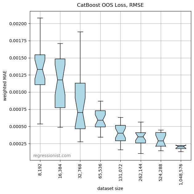
CatBoost requires a pretty large dataset size to produce a good fit for data this noisy. Compared to using polynomial regression, this model is clearly not as accurate. Here is an example of the fit for our largest dataset size:
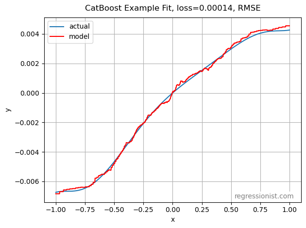
This is clearly not a perfect model. We run the optimization process again with MAE as our loss function to see if we can get a better model. Here is the plot of mean error:
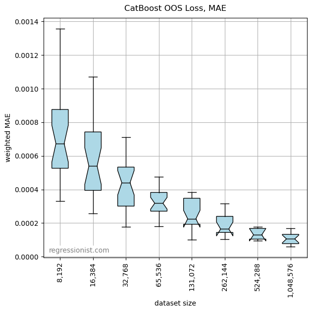
This is marked improvement. Here is an example fit from our largest dataset size:
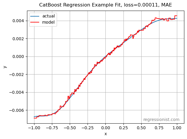
Lastly, we want to know how the monotonicity constraint changes our model. Here we see the mean OOS loss:
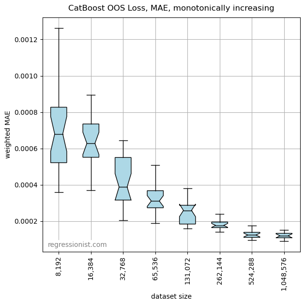
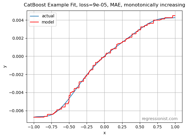
This appears to be very similar to the accuracy of the model without the monotonicity constraint. Here we look at an example of the model for our largest dataset:
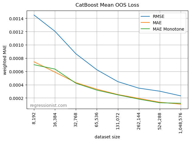
We can get a good feel for the comparative performance of these hyperparameter settings by plotting the mean OOS loss for each dataset size:
Conclusion
CatBoost can be a useful algorithm for modeling noisy financial data, but we can see the importance of hyperparameter tuning. Changing just the log loss parameter from the default RMSE function to the MAE function significantly impacts the performance of the model. It appears that for this data, the monotonicity constraint doesn’t have a large effect on the accuracy of the model.
Impressively, despite the disadvantage of not being provided with the weights of the data during training, CatBoost still provides a very good model. For the dataset sizes we tried and when using MAE, this algorithm outperforms a polynomial regression model, further highlighting CatBoost’s capabilities in handling regression problems.
References
- “Benchmarks.” CatBoost, https://catboost.ai/#benchmark.
- Dorogush, Anna Veronika. “Anna Veronika Dorogush – CatBoost – the new generation of Gradient Boosting.” YouTube, uploaded by EuroPython Conference, Aug. 30, 2018, https://youtu.be/oGRIGdsz7bM.