We need simple synthetic data with known structure that will allow us to visually compare what models learn against the ground truth. This data will be used to evaluate and compare machine learning algorithms, so it is important for it to closely simulate real-world data one might might actually care about. We will use synthetic rather than real data, however, because it helps to know the true generating function when evaluating over- or under-fitting. Additionally, we’re going to need quite a lot of this data, since we will run many simulations as part of each experiment.

Generating Function

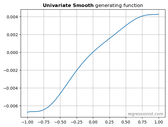
The generating function is intended to resemble signals found in simple intraday stock prediction models. The scale is reasonable, ranging from -67 bps to 43 bps. The shape is basically monotonic, nonlinear, asymmetric, and flattens out at the ends. We found the formula by plugging a few points into an online polynomial fitting tool.

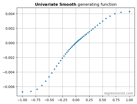
The strongest signals tend to be more rare. So we’re going to choose x-values from a non-uniform distribution. We’re going to sample x from a Laplace distribution centered at 0 with scale parameter 0.4. This scatterplot of the generating function shows the lower density of x-values at the edges.

Realistic Noise

The distribution of asset returns is an evergreen topic of study due to its relevance in option pricing. However, for simplicity, we will just use whatever distribution in SciPy most reasonably describes actual historical stock returns.

This synthetic dataset is meant to simulate intraday stock returns – a little signal and a lot of fat-tailed noise. To get the noise right, we looked at the distribution of simple intraday returns (close_t / open_t - 1) of all US equities trading over $5 million a day, for the past four years. We then followed Martin’s advice for finding the best-fitting of all the SciPy continuous distributions. The winner was Student’s t-distribution, with the PDF:
f(x) = \frac{\Gamma((\nu + 1)/2)}{s \sqrt{\pi \nu} \Gamma(\nu / 2)} (1 + (x/s)^2 / \nu)^{-(\nu + 1) / 2}
Where the calibration found the degrees of freedom:
\nu = 1.875
and the scale factor:
s = 0.0123

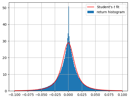
The fit isn’t perfect. However, it is pretty good in the tails. It might even be conservative, since it downweights the sharp spike near 0 and gives that weight to the [0.01-0.02] region, effectively adding more noise.

Putting it Together

Here is the complete code for combining the signal with the noise to create a synthetic data sample:

import time
import numpy as np
import scipy.stats
np.random.seed(time.time_ns() % 1000000)

m = 100 # number of examples

# hypothetical feature value x
# start with twice as many as needed
x = scipy.stats.laplace.rvs(loc=0, scale=0.4, size=2*m)

# rejection sampling to truncate range to (-1, 1)
x = x[np.where(np.abs(x) < 1)][:m]

# signal generating function
g = np.polynomial.Polynomial([0,
                              6.8236382645559986e-003,
                             -4.7065634351623866e-003,
                              6.7041461913671437e-003,
                              5.9494959647700936e-003,
                             -1.5600272408065097e-002,
                             -2.4815593030551139e-003,
                              7.5757817838128481e-003])
signal = g(x)

# noise simulating liquid equity intraday returns
# start with twice as many as needed
nu = 1.8752571511115708
scale = 0.012289408564391225
noise = scipy.stats.t.rvs(nu, loc=0, scale=scale, size=2*m)

# rejection sampling to truncate noise range to (-1, 1)
# max drawdown -100%, max positive return 100%
# to make it a little easier for the ML algorithms
noise = noise[np.where(np.abs(noise) < 1)][:len(x)]

y = signal + noise

Here is an example plot to see what the data looks like:

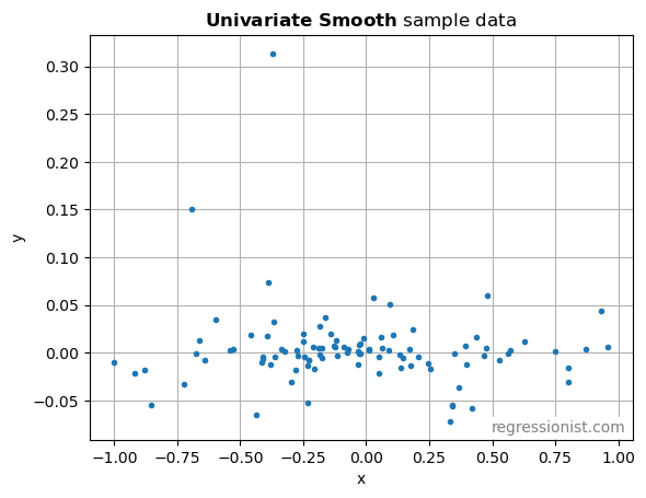
Clearly, an algorithm would struggle to pick out the signal in such noisy data with only these 100 points. But that is the nature of financial data.

Evaluation Criterion

A simple trading strategy based on the structure in this data would only trade when the expected edge was higher than the transaction costs. So the many small forecasts would be uninteresting. What matters is that the forecasts are accurate when they are high. As we evaluate different machine learning algorithms, we’re going to overweight prediction error in the regions of interest where |x| is large:

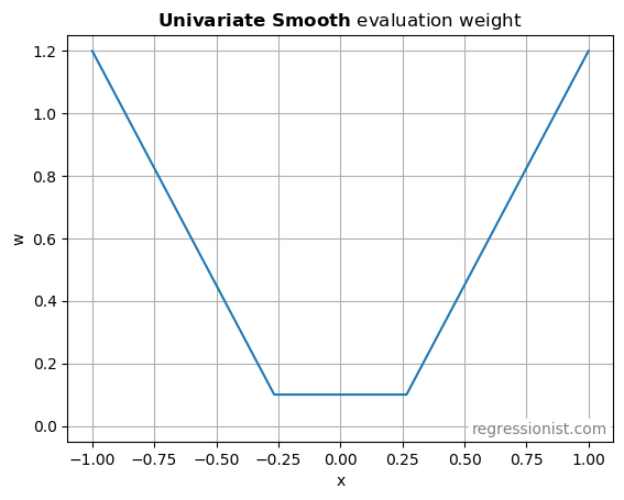
Also, we’re going to use weighted mean absolute error (MAE) instead of mean squared error (MSE). Because a bad trade loses money linearly, and not quadratically. So the evaluation criterion for model predictions on this dataset will be:

x = np.linspace(-1, 1, 1000)
signal = g(x)
pred = model.predict(x)
w = np.maximum(1.5 * np.abs(x), 0.4) - 0.3
MAE = np.sum(w * np.abs(pred - signal)) / np.sum(w)