When creating a model on data we expect to be noisy, choosing the right error function can have a huge effect on model performance. Some loss functions heavily penalize large errors and outliers while others give them less weight when creating the final model.

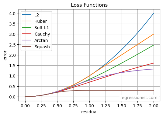
A few loss functions used in regression are defined as follows, with y as the observed value and \hat{y} as the predicted value:

• L2: \quad\sum_{i=1}^n (y_i - \hat{y}_i)^2
• Soft L1: \quad\sum_{i=1}^n 2(\sqrt{1 + (y_i - \hat{y}_i)^2} - 1)
• Cauchy: \quad\sum_{i=1}^n \ln(1 + (y_i - \hat{y}_i)^2)
• Arctan: \quad\sum_{i=1}^n \arctan((y_i - \hat{y}_i)^2)
• Huber: \text{error} = \sum_{i=1}^n f(y_i - \hat{y}_i), \quad f(y_i - \hat{y}_i)=\begin{cases} \frac12 (y_i - \hat{y}_i)^2 \quad &\text{if} \, y_i - \hat{y}_i \leq \sigma \\ \sigma (|y_i - \hat{y}_i| - \frac{\sigma}{2}) \quad &\text{if} \, y_i - \hat{y}_i > \sigma \end{cases}

We may also use a custom squashing function on any loss function that puts a limit on the size of the penalty. Here we define a smooth squashing function:

The value k is a parameter that we may adjust, allowing us to change the amount of squashing we want to induce on our residual calculations. Below is a graph of the squashing function with k=0.1:

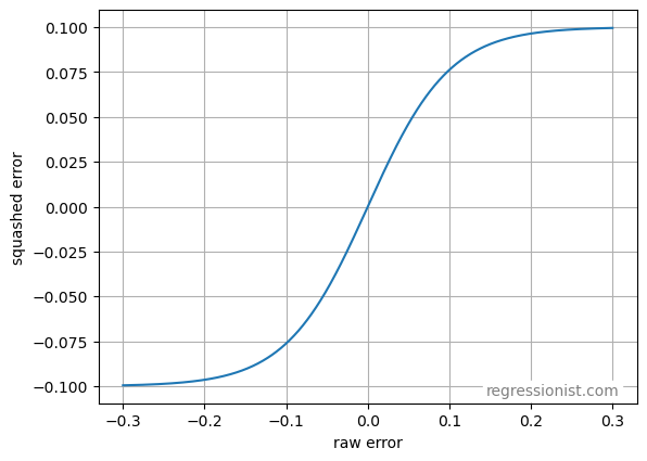
Then for any value of k, any given datapoint can have an error of no more than k. In this way, we can bound the size of the penalty and prevent excessive weighting of large errors.

In this article, we compare the results of models made with each of these loss functions.

Regression Methods

>>> scipy.optimize.least_squares

One package for predictive modeling with different loss functions built in is scipy.optimize.least_squares. This has the handy option of accepting an argument in the parameters to determine which of several loss functions to use (linear, Huber, soft_l1, cauchy, and arctan). The linear option is the L2 loss described above, and the implementation of Huber loss uses a \sigma = 2 . It is important to note that the least_squares method squares residuals before the loss function is applied — meaning it uses the mathematical definitions from above.

By default, scipy.optimize.least_squares performs non-linear least squares, but because our purpose here is simply to compare loss functions, we use a less computationally expensive linear model. We may do this by changing the way we calculate our residuals:

# Calculate residuals
def residual_function(x, *args, **kwargs):
     prediction = x[0] + x[1] * data['X_train'].flatten()
     return data['y_train'] - prediction

This is the residual function we pass to the least_squares method as the ‘fun’ parameter. The least_squares method then returns the optimum value of x, which is a list of two elements defining the y-intercept and slope of a line.

We then make an initial estimate and create a model and prediction as follows:

# Initial guess
x0 = [0,0]

# Model and prediction
ls = least_squares(fun=residual_function, x0=x0, loss='linear', gtol=1e-12, xtol=1e-12, ftol=1e-12)   
pred = ls.x[0] + ls.x[1] * data['X_test'].flatten()

We have also lowered our default tolerance values to provide greater accuracy.

>>> scipy.optimize.minimize

Another method that allows us to use the same loss functions without squaring the residuals is scipy.optimize.minimize with custom loss functions. The process is nearly identical as the steps followed above, but we redefine the loss functions to use the absolute value of the residual instead of the square.

Experiment Design

We test the usefulness of different loss functions and error squashing using the noisy univariate smooth dataset.

For each dataset size from 4,000 to 24,000 (stepping by increments of 2,000), we make 100 new synthetic datasets. For each of these 1,100 datasets, we create a model with each of the loss function options in scipy.optimize.least_squares. We also create a model on each of the datasets using the same loss functions, but with our redefined loss functions in scipy.optimize.minimize in order to avoid squaring the residuals. We also use Scipy’s minimize to create a model with the smooth squashing loss function for both squared and non-squared residuals. We then find the average MAE all the models of the given size. In this way, we test the same loss functions on squared and non-squared residuals.

One final note is that each time the experiment code is run, we use skopt.forest.minimize to optimize the parameters \sigma (for the Huber loss with non-squared residuals) and k (for the smooth squashing loss function with separate optimization for squared and non-squared residuals). We do this by performing 50 calls to an objective function for each of the optimization problems. For k, we search uniformly on the interval [0.01, 0.2] , and for sigma the uniform interval [0.001, 0.5] .

Results

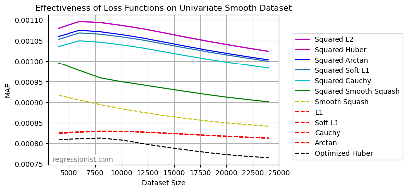
First, we obtain a table of the average MAE for models on each dataset size:

Here we see a graphical representation of the same data:

Below is a plot of a model made with the optimized optimized Huber loss function on non-squared residuals at our largest dataset size:

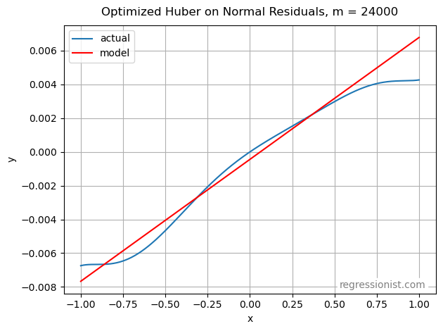
This model provides a wonderful fit for a linear approximation.

Conclusion

Note that some of the loss functions graphed yield nearly identical results. It is unsurprising that Scipy’s L2 and Huber losses from the least_squares method were so similar, because the sigma value used is 2, and with the way our data is scaled very few residuals will reach this magnitude. Then Huber loss on squared residuals will always be essentially the same as L2 loss on squared residuals for data of this scale when using least_squares.

Additionally, every loss function we tried yielded better results on this data when applied to residuals as opposed to squared residuals. In fact, most of the loss functions (L1, soft L1, Cauchy, and arctan) had nearly identical performance to each other when residuals were not squared. These error functions also proved to be very effective even at small dataset sizes, performing at a very similar level on smaller amounts of data as on larger amounts.

Interestingly, smooth squashing was by far the superior choice when performed on squared residuals, but with ordinary residuals, it was the least effective.

Finally, our winning function was the optimized Huber on non-squared residuals. When eliminating squared residuals, the loss function becomes discontinuous at \sigma . In our experiments, the \sigma value chosen was generally close to 0.1, creating a larger penalty for observations with residuals less than \sigma, followed by a drop-off to a more gradual increase in penalty size for larger residuals.

While any of the above loss functions will give good results, when accuracy really matters, it is clear to see that our choice can have a measurable impact on our model. This experiment will aid us in choosing loss functions for future models and highlights the importance of testing different types of error calculation in predictive modeling.