
The main lesson we learned working with the Univariate Smooth data was that fat tails were very challenging for the different learning algorithms, but that the tails could be tamed prior to learning through squashing. So this new synthetic data will not focus on fat tailed noise, but will instead focus on complex nonlinear structure.
Generating Function
The generating function is composed of univariate functions of synthetic features:
\begin{aligned} y =& f_1(x_1) \cdot f_2(x_2) \cdot f_3(x_3) \\ +& f_4(x_4) \cdot f_5(x_5) \\ +& f_6(x_6) \\ +& 0 \cdot x_7 \\ +& 0 \cdot x_8 \\ +& 0 \cdot x_9 \\ +& \epsilon \end{aligned}Note that the last three features have no effect on y and are only included to test how well learning algorithms handle superfluous features.
f_1(x_1)
Draw x_1 randomly from a normal distribution, and run it through a tanh function:
x_1 \sim \mathcal{N}(0,1) f_1(x) = 0.001 \cdot \text{tanh}(x)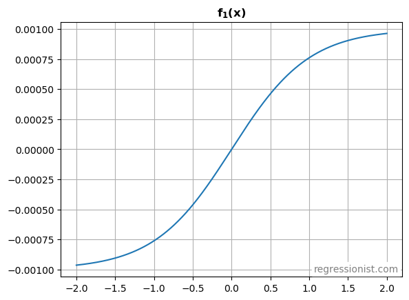
f_2(x_2)
Draw x_2 randomly from a uniform distribution, and run it through a linear function:
x_2 \sim \mathcal{U}_{[-1,1]} f_2(x) = 1 - 0.5x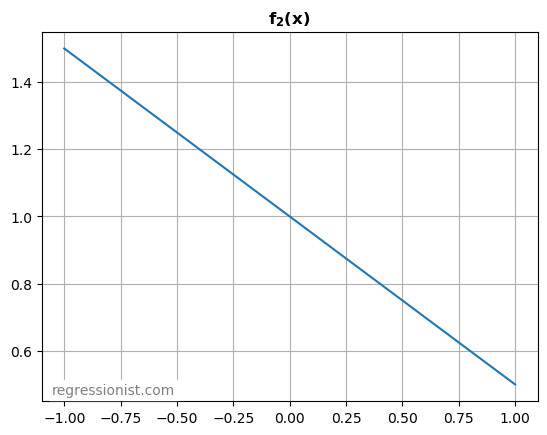
f_3(x_3)
Draw x_3 randomly from a discrete set of values {-1, 0, 1} such that:
\begin{aligned} &\mathbb{P}(x_3=-1) = 0.25 \\ &\mathbb{P}(x_3=0) = 0.55 \\ &\mathbb{P}(x_3=1) = 0.2 \end{aligned} f_3(x) = \begin{cases} 0.6 &\text{if } x = -1 \\ 1 &\text{if } x = 0 \\ 1.5 &\text{if } x = 1 \end{cases}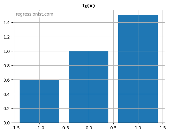
f_4(x_4)
Draw x_4 randomly from a uniform distribution:
x_4 \sim \mathcal{U}_{[0,1]} f_4(x) = 0.0008 x^{0.6}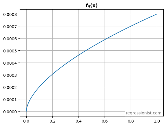
f_5(x_5)
Draw x_5 randomly from a normal distribution, and run it through a sine function:
x_5 \sim \mathcal{N}(0,1) f_5(x) = 1 + 0.5 \cdot \text{sin}(x)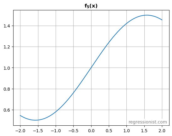
f_6(x_6)
Draw x_6 randomly from a normal distribution, but make it highly correlated with x_1:
x_6 \sim \mathcal{N}(0,1)\ \text{s.t.} \\ \text{cov}(x_1, x_6) = 0.85 f_6(x) = \left(\frac{1}{700} \right) \cdot \left(\frac{1}{1+e^{-|3x|}} - 0.5 \right)^{0.5}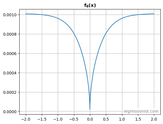
x_7,\ x_8,\ x_9
Draw x_7 randomly from a normal distribution:
x_7 \sim \mathcal{N}(0,1)Draw x_8 randomly from a uniform distribution:
x_8 \sim \mathcal{U}_{[-1,1]}Draw x_9 randomly from a discrete set of values {-1, 0, 1} such that:
\begin{aligned} &\mathbb{P}(x_9=-1) = 0.1 \\ &\mathbb{P}(x_9=0) = 0.6 \\ &\mathbb{P}(x_9=1) = 0.3 \end{aligned}Noise
Draw \epsilon randomly from a normal distribution to provide noise similar to the distribution of simple intraday stock returns, but without fat tails:
\epsilon \sim \mathcal{N}(0,0.02)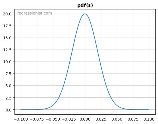
Putting it Together
Here is the complete code for combining the signal with the noise to create a synthetic data sample:
import time
import numpy as np
import scipy.stats
np.random.seed(time.time_ns() % 1000000)

m = 100 # number of examples

# prepare random variables (with x1 correlated with x6)
mu = np.array([0., 0.])
Sigma = np.array([
            [ 1.00, -0.85],
            [-0.85,  1.00]
        ])
Xc = np.random.multivariate_normal(mu, Sigma, size=m)
x1 = Xc[:,0]
x6 = Xc[:,1]
x2 = np.random.uniform(-1, 1, m)
p = np.random.uniform(0, 1, m)
x3 = np.zeros(p.shape)
x3[p <= 0.25] = -1
x3[p > 0.8] = 1
x4 = np.random.uniform(0, 1, m)
x5 = np.random.normal(0, 1, m)
x7 = np.random.normal(0, 1, m)
x8 = np.random.uniform(-1, 1, m)
p = np.random.uniform(0, 1, m)
x9 = np.zeros(p.shape)
x9[p <= 0.1] = -1
x9[p > 0.7] = 1

# noise is normally distributed
epsilon = np.random.normal(0, 0.02, m)

# calculate function values
f1 = 0.001 * np.tanh(x1)
f2 = 1 - 0.5 * x2
f3 = np.ones((m,))
f3[x3 == -1] = 0.6
f3[x3 == 1] = 1.5
f4 = 0.0008 * x4**(3/5)
f5 = 1 + 0.5 * np.sin(x5)
f6 = np.sqrt(1 / (1 + np.exp(-np.abs(3 * x6))) - 0.5) / 700

# combine into a signal
signal = f1*f2*f3 + f4*f5 + f6

# add noise
y = signal + epsilon

# build design matrix
X = np.column_stack([x1, x2, x3, x4, x5, x6, x7, x8, x9])
Evaluation Criterion
We’ll stick with uniform weighting this time. But we will continue to use mean absolute error (MAE) instead of mean squared error (MSE). Again, because a bad trade loses money linearly, and not quadratically. So the evaluation criterion for model predictions on this dataset will be:
MAE = np.mean(np.abs(pred_test - signal_test))